We introduced in a previous post a library for operating with arbitrarily big numbers, where we implemented some basic arithmetic operations, like addition, multiplication and division.

In this post we will focus on improving the efficiency of the multiplication algorithm through Fast Fourier Transforms.

The algorithm

Let’s take two random numbers, say

$$\begin{array}{c} a = 143672,\\ b = 669381 \end{array}$$

The multiplication result is

$$a \cdot b = 96171307032$$

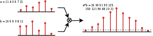
If we see each number as a digit sequence (digits between 0 and 9), we can think of each of those digits as coefficients of a polynomial. The multiplication of two polynomials and the ordinary multiplication are closely related

$$\begin{array}{c} p_a(x) = x^5+4\,x^4+3\,x^3+6\,x^2+7\,x+2\\ p_b(x) = 6\,x^5+6\,x^4+9\,x^3+3\,x^2+8\,x+1 \end{array}$$ $$\begin{array}{c} p_a(x) \cdot p_b(x) = 6\,x^{10} + 30\,x^9 + 91\,x^8 + 53\,x^7 + 125\,x^6 + 150\,x^5 + \\ 121\,x^4 + 90\,x^3 + 68\,x^2 + 23\,x + 2 \end{array}$$

Thus, we obtain the sequence [6 30 91 53 125 150 121 90 68 23 2]. As some of these digits are greater than 9, we need to apply a carry propagation correction, obtaining the sequence [9 6 1 7 1 3 0 7 0 3 2], which is the result we were looking for. The carry correction algorithm has a time complexity of order $O(n)$.

It is well known that a polynomial multiplication algorithm is equivalent to a discrete convolution over the coefficients, so we can also conceive our digit sequences as discrete signals.

The discrete convolution can be computed as

$$(a * b)[n] = \displaystyle{\sum_{m=-\infty}^{\infty}{a[m] \cdot b[n-m]}}.$$

The classical algorithm for the convolution has an order of $O(n^2)$ time complexity, so there is no point at the moment. To reduce this complexity, we’ll use the convolution theorem, which tells us that the Fourier transform of a convolution is the pointwise product of the Fourier transforms.

$$\mathcal{F}\{a * b\} = \mathcal{F}\{a\} \cdot \mathcal{F}\{b\}.$$

That is, we can compute the DFTs of the original signals, multiply them pointwise, compute the inverse DFT and apply the decimal correction. The key point is that we can use efficient FFT algorithms to compute both the DFT and the inverse DFT.

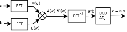
From a $O(n^2)$ order algorithm, we have moved to the computation of two FFTs, with order $O(n \cdot log_2(n))$ each one, a pointwise product, with $O(n)$, an inverse FFT, with $O(n \cdot log_2(n))$, and a carry propagation correction, with $O(n)$, so putting all together, our final algorithm will have an order of $O(n \cdot log_2(n))$, much better than the original algorithm.

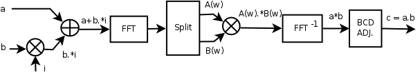
As a final optimization, it is possible to avoid computing one of the two FFTs if we take into account that the original signals are both real, so if we build a complex signal which carries one of the signals in its real part and the other signal in the imaginary part

$$c[n] = a[n] + i\,b[n],$$

we can extract the original signals applying the real part and imaginary part operators

$$\begin{array}{c} a[n] = \Re\{y[n]\} = \dfrac{c[n] + c^*[n]}{2}\ \\ b[n] = \Im\{y[n]\} = \dfrac{c[n] - c^*[n]}{2\,i} \end{array}.$$

Using the following property of the Fourier transform

$$a^*[n] \longrightarrow \mathcal{F}\{a\}^*[-n],$$

we can compute now the DFT of the composite signal and extract the DFTs of the original signals

$$\begin{array}{c} \mathcal{F}\{a\}[n] = \dfrac{\mathcal{F}\{c\}[n] + \mathcal{F}\{c\}^*[-n]}{2}\ \\ \mathcal{F}\{b\}[n] = \dfrac{\mathcal{F}\{c\}[n] - \mathcal{F}\{c\}^*[-n]}{2\,i} \end{array},$$

where the extra operations have all order $O(n)$.

The code

Starting from the original code, some functions have been added: FFT and inverse FFT computation functions, in the files fft.h and fft.c. Also, the memory allocation is now dynamic in order to deal with really huge numbers; furthermore, the show() function has been improved in such a way that it only prints the most and less significant digits with very big numbers, while the whole computation is dumped to the file output.txt.

To test the new multiplication algorithm, the program evaluates the largest known prime number at the moment this post was written, the Mersenne prime $2^{43,112,609}-1$, with 12,978,189 digits. You no longer need to modify BigNumber::N_DIGITS, it will automatically adapt to the selected exponent. In this case, we need $2^{24}$ = 16,777,216 figures - must be power of 2 - to compute a number with 13 million digits.

The algorithm used to obtain the Mersenne number is detailed in the source code. You will need a few minutes and 1,3 GB of RAM memory to run the program with the current configuration in a normal - as of 2010 - computer. If that’s too long for you, you can compute a cheaper Mersenne prime, e.g. the number $2^{3,021,377}-1$ (with 909,526 digits), in a few seconds.

Take a look to those humongous numbers to get an idea of what we are talking about. Find below the execution output for both of them in raw text formatted to 75 columns. Can you imagine how hard it must be to proof that they are indeed prime numbers?

• Output for Mersenne prime number $2^{3,021,377}-1$
• Output for Mersenne prime number $2^{43,112,609}-1$

It is possible to aplly some improvements with parallelization and a more dynamic memory allocation, but that’s beyond the scope of this post. In future articles we will introduce algorithms to perform more complicated mathematical operations, like square roots.

Links

• Library hosted on github.com (the code explained here is tagged as 1.0.1, the posterior code can contain improvements explained in future posts)
• Source code