Modeling and simulation of planetary motion

One of my favourite problems in classical mechanics is the planetary motion, and one of my first attempts to solve it with computer algorithms dates from my early teens. My first approach was written in BASIC, and the results were completely wrong, as I didn’t know enough about the underlying maths. Subsequent attempts produced good results once I knew some basics of differential calculus during my high-school years.

In this post I’ll rescue one of those implementations, written in C, which uses the laws of motion to compute astronomical body paths.

Physics background

Let’s suppose we have two bodies $B_1$ and $B_2$ , at positions $\vec{p}_1$ and $\vec{p}_2$ , and with masses $m_1$ and $m_2$ , respectively. Newton’s law of universal gravitation states that the force between the two bodies is proportional to the product of the two masses, and inversely proportional to the squared distance:

$F = G\,\dfrac{m_1 \cdot m_2}{r^2}.$

Where $r = \left|\vec{p}_1-\vec{p}_2\right |$ . For instance, the force with which $B_1$ is attracted towards $B_2$ , including magnitude and direction, and being $\hat{r}$ the unitary vector from $\vec{p}_1$ to $\vec{p}_2$ , is

$\vec{F}_{12} = G\,\dfrac{m_1 \cdot m_2}{\left|\vec{p}_1-\vec{p}_2\right|^2}\hat{r} = G\,\dfrac{m_1 \cdot m_2}{\left|\vec{p}_1-\vec{p}_2\right|^3}(\vec{p}_2-\vec{p}_1)$

Figure 1: Solution example when two bodies interact.

If we also use Newton’s second law of motion, which relates force and acceleration

$\vec{F} = m\,\vec{a},$

and knowing that the acceleration $\vec{a}(t)$ is the second time derivative of position $\vec{p}(t)$

$\vec{a}(t) = \dfrac{d^2}{dt^2}\vec{p}(t),$

we can express the problem with the following set of coupled non-linear differential equations:

$\begin{array}{c} \dfrac{d^2}{dt^2}\vec{p}_1(t) = G\,\dfrac{m_2}{\left|\vec{p}_1(t)-\vec{p}_2(t)\right|^3}(\vec{p}_2(t)-\vec{p}_1(t))\\ \dfrac{d^2}{dt^2}\vec{p}_2(t) = G\,\dfrac{m_1}{\left|\vec{p}_1(t)-\vec{p}_2(t)\right|^3}(\vec{p}_1(t)-\vec{p}_2(t)). \end{array}$

If we provide the initial conditions, i.e. the initial positions $\vec{p}_1(t_0)$ and $\vec{p}_2(t_0)$ , and the initial velocities $\vec{v}_1(t_0)$ and $\vec{v}_2(t_0)$ , we can obtain, from the above equations, the paths $\vec{p}_1(t)$ and $\vec{p}_2(t)$ , regardless of the number of dimensions. Particularly, for a two-dimensional problem, where

$\begin{array}{c} \vec{p}_1(t) = (x_1(t), y_1(t))\\ \vec{p}_2(t) = (x_2(t), y_2(t)), \end{array}$

the set of equations becomes

$\begin{array}{c} \dfrac{d^2}{dt^2}x_1(t) = G\,\dfrac{m_2}{\bigl((x_1(t)-x_2(t))^2+(y_1(t)-y_2(t))^2\bigr)^\frac{3}{2}}\bigl(x_2(t)-x_1(t)\bigr)\\ \dfrac{d^2}{dt^2}y_1(t) = G\,\dfrac{m_2}{\bigl((x_1(t)-x_2(t))^2+(y_1(t)-y_2(t))^2\bigr)^\frac{3}{2}}\bigl(y_2(t)-y_1(t)\bigr)\\ \dfrac{d^2}{dt^2}x_2(t) = G\,\dfrac{m_1}{\bigl((x_1(t)-x_2(t))^2+(y_1(t)-y_2(t))^2\bigr)^\frac{3}{2}}\bigl(x_1(t)-x_2(t)\bigr)\\ \dfrac{d^2}{dt^2}y_2(t) = G\,\dfrac{m_1}{\bigl((x_1(t)-x_2(t))^2+(y_1(t)-y_2(t))^2\bigr)^\frac{3}{2}}\bigl(y_1(t)-y_2(t)\bigr), \end{array}$

Figure 2: Same solution as before, but showing the relative motion. The result is an ellipse.

where we have to find $x_1(t)$ , $y_1(t)$ , $x_2(t)$ and $y_2(t)$ . The problem can be easily generalized to $N$ dimensions and $M$ bodies.

Designing an numerical method to solve the equations

If we discretize the time domain

Figure 3: 3D solution example.

$t_n = t_0 + n\,\Delta_t\,\qquad n \in \mathbb{Z}^+,$

and we apply the following first order finite differences approximations of the differential operators (this is the easiest way, and it’s equivalent to Euler method):

$\begin{array}{c} \vec{v}(t) = \dfrac{d}{dt}\vec{p}(t) \simeq \dfrac{\vec{p}(t+\Delta_t)-\vec{p}(t)}{\Delta_t}\\ \vec{a}(t) = \dfrac{d}{dt}\vec{v}(t) \simeq \dfrac{\vec{v}(t+\Delta_t)-\vec{v}(t)}{\Delta_t} \end{array}$

We can compute both the velocity and position of a body $B_i$ , given the force exerted over it, by finding $\vec{p}_i(t+\Delta_t)$ from the above equations

As simple as:

We compute the forces for each body (the forces due to all the other bodies): $\vec{F}_i = \displaystyle\sum_{j \neq i}G\,\dfrac{m_i \cdot m_j}{\left|\vec{p}_i(t_n)-\vec{p}_j(t_n)\right|^3}\bigl(\vec{p}_j(t_n)-\vec{p}_i(t_n)\bigr)$
Hence we have the acceleration over each body: $\vec{a}_i = \dfrac{\vec{F}_i}{m_i}$
We integrate it, once to obtain the velocity: $\vec{v}_i(t_n+\Delta_t) = \vec{v}_i(t_n) + \Delta_t\,\vec{a}_i$
And we integrate it again, for the position: $\vec{p}_i(t_n+\Delta_t) = \vec{p}_i(t_n) + \Delta_t\,\vec{v}_i(t_n)$

The code

In the link below you have an implementation in C for the two-dimensional case. The code is ancient and platform-dependent, as it uses some basic graphic routines. Originally this code was written for MS-DOS, using the protected mode and the mode 13h. The code was originally compiled with the DJGPP programming platform under RHIDE. As this platform is from the past, you can either run it under an emulator like DOSBox, or compile it using the SDL wrapper that I’ve written for rescuing this and other old code (only tested under GNU/Linux). The wrapper is implemented in files mode13h.h and mode13h.c (the only platform-dependent code), and in order to switch between a native MS-DOS platform and SDL you must use the DOS symbol (when present, it assumes a native MS-DOS platform, otherwise it will use SDL).

The main algorithm is implemented in file newton.c, and, as I described before, it just computes the force exerted over each body, and then velocity and position.

Figure 4: Example of execution with relative motion.

A body is modelled with the struct body_t, which considers the position and velocity. Before starting the algorithm, you must create the bodies with the createBody() function, providing initial position, initial velocity and mass. Also, you can specify whether or not the body is fixed at its position, to simulate fictitious situations, suitable to being validated against Keppler’s laws (you can visually check how the two first laws hold when only two bodies interact). Another way to do this with real cases is by using the bodyref variable: when this variable is not null, the camera will follow the selected body.

Other useful parameters are scale_factor, to fit the required space in the screen, and calculations_per_plot, that allows you to enable frame dropping, computing with enough accuracy without having to plot all the solutions.

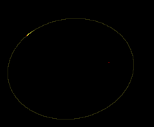
The source code includes an example of an Earth–Moon system, where you can check that, given realistic data for the initial values and masses, some other parameters like the orbital period match the known values.

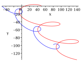
In this video you can watch an execution example of the three-body problem, under DOSBox emulator, where you can appreciate the chaotic behaviour.

Links

Written on December 5, 2011